

Control selection
This section explains how IMPC selects and groups data for statistical analysis, how mutant measurements are compared with wild-type controls, and how soft windowing prioritises controls collected close in time to the mutant observations. It covers:
Control selection strategy
One side effect of producing data in a high throughput pipeline is that the input data for a statistical calculation might be produced over multiple days. Environmental fluctuations have been identified as a confounding factor when comparing data gathered on different days. The IMPC describes this as a “batch effect” and it is treated as a random effect in the mixed-model framework.
The data sets to be analysed are identified using unique combinations of these fields:
| Field | Description |
|---|---|
| Background strain | The original strain from which the mutant specimen was derived. |
| Allele / Colony | The genomic variation in the mutant. The allele describes the character and the severity of the mutation. |
| Zygosity | WT (wild-type or +/+) The wild-type allele. Heterozygous (het) The mutation occurred in one copy of the allele. Homozygous (hom) The mutation occurred in both copies of the allele. Hemizygous (hemi) The mutation occurred in a sex-linked allele where, normally, only a single copy exists in the WT. |
| Pipeline | The standardised phenotyping pipeline as described in IMPReSS pipelines. |
| Procedure | The standardised set of procedures (experiments) as described in IMPReSS procedures. |
| Parameter | The standardised set of measurements as described in IMPReSS parameters. |
| Metadata group | Some parameters are indicated as “procedureMetadata” type. Some of these metadata are used to group comparable data together as described on the IMPReSS parameters page under the “Required For Data Analysis” section. The parameters that are marked as “Required For Data Analysis” are collectively identified by an identifier called the metadata group. |
| Organisation | The phenotyping facility where the experiments were performed and the data collected. |
| Sex* * – optional | The sex of the specimens. In the linear mixed-model analysis, males and females are analysed together, allowing the analysis to estimate the Sex and Sex × Genotype interaction effects. If required, sex can also be included as an additional grouping term to produce sex-specific results. |
Relevant reading:
Please see this IMPC paper on a soft windowing application to improve analysis of high-throughput phenotyping data, Bioinformatics 36, 1492–1500 (2020).
Soft windowing
All IMPC statistical analyses compare observations in genetic mutant animals against observations of wild-type controls.
The IMPC protocols guarantee that all mutant measurements are accompanied by corresponding data from matched non-mutant animals, i.e. from animals assessed at the same time and at the same facility. As a result, the IMPC has a large collection of measurements pertaining to wild-type animals, all of which are annotated with metadata.
Although the wild-type data have some variability, as power analyses have shown, statistical tests benefit from using a wide set of control data points. Thus, unless the control metadata indicate substantial changes, mutant lines are compared against controls from their immediate control group as well as many other relevant animals. In practice, the effective control pool can include up to several thousand wild-type animals.
Changes in metadata that disqualify pooling controls include differences in location (mutants are compared only against wild-type animals processed at the same facility).
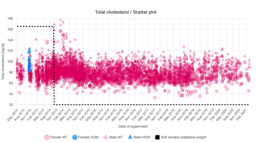
Since Data Release 15.1, the IMPC implements a soft windowing procedure. Each eligible control mouse is given a statistical weight based on how close in time it was measured to the mutant mice: nearby controls have greater influence on the comparison, while more distant controls have less. This gives recent controls more relevance without requiring a rigid date cutoff.
In the current implementation, soft windowing is applied only to numeric parameters analysed using the linear mixed model. If the calculated weights have fewer than two unique values or their variance is below the soft-window threshold of 1.4901 × 10⁻⁷, the standard non-windowed model is used instead. When more than 15 unique mutant experiment dates are available for the windowing calculation, 15 dates are randomly sampled.
This soft windowing threshold is calculated in the current statistical pipeline as an R expression: sqrt(.Machine$double.eps) * 10. This is the square root of machine epsilon multiplied by ten. It is a small numerical cutoff to exclude negligible soft-windowing weights and keep model fitting numerically stable.
The comparison is strictly greater than the threshold. The displayed value, 1.4901 × 10⁻⁷, is rounded to four decimal places in scientific notation; the statistical pipeline uses the unrounded threshold defined above.
Zero is not used as the threshold because soft windowing assigns weights using a smooth function. Measurements far from the mutant experiment dates usually receive very small positive weights rather than exactly zero. If the threshold were zero, these distant measurements would still be included in the model. The non-zero threshold treats numerically negligible weights as zero and prevents numerical problems when the model uses the inverse of the weight.
The window_weight reflects the importance assigned to each measurement based on how close its experiment date is to the mutant experiment dates. The pipeline uses batch dates for this comparison. Dates near a mutant date receive larger weights. Where windows around several mutant dates overlap, their effects are combined. By default, the weighting curve is logistic, and the software adjusts the window width and steepness by trying different settings.
The weights then affect how much each observation contributes to the final model: higher-weight observations count more, and very small weights may be excluded. Sex and body weight can be included in the model, but they do not determine the weights.
Learn more:
- The soft windowing approach is discussed in a news post.
- Further details are available in the soft windowing paper, Bioinformatics 36, 1492–1500 (2020).
- Power analysis is described in this paper.
How to identify the controls used in a soft-windowed analysis
The data underlying an analysis can be downloaded in TSV or XLS format from the relevant chart page. The download includes all mutant and control observations, including those not used in the final soft-windowed statistical model. Use the window_weight column to identify controls that pass the soft-windowing weight filter, as described below.
To identify the controls included in the model:
- Select rows where
biological_sample_groupiscontrol. - Exclude rows where
window_weightis blank or missing. - Retain rows where:
window_weight > 1.4901 × 10⁻⁷
| window_weight | Interpretation |
|---|---|
| Missing | No soft-windowing model weight was assigned |
| Less than or equal to 1.4901 × 10⁻⁷ | Weight was calculated, but the observation was excluded from the final model |
| Greater than 1.4901 × 10⁻⁷ | Observation was included in the final soft-windowed model |